How should we model surpluses and deficits? In finishing up a recent articleand chapter 5 and 6 of a Fiscal Theory of the Price Level update, a bunch of observations coalesced that are worth passing on in blog post form.

Background: The real value of nominal government debt equals the present value of real primary surpluses, [ frac{B_{t-1}}{P_{t}}=b_{t}=E_{t}sum_{j=0}^{infty}beta^{j}s_{t+j}. ] I ‘m going to use one-period nominal debt and a constant discount rate for simplicity. In the fiscal theory of the price level, the (B) and (s) decisions cause inflation (P). In other theories, the Fed is in charge of (P), and (s) adjusts passively. This distinction does not matter for this discussion. This equation and all the issues in this blog post hold in both fiscal and standard theories.

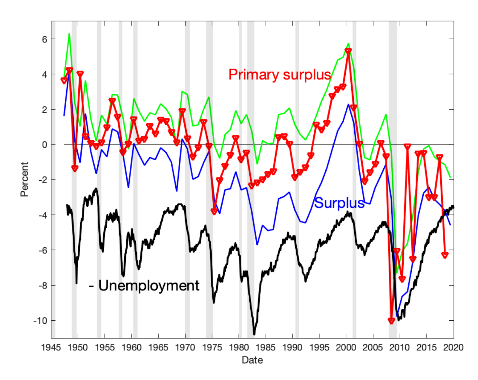
The question is, what is a reasonable time-series process for (left{s_{t}right} ) consistent with the debt valuation formula? Here are surpluses

The blue line is the NIPA surplus/GDP ratio. The red line is my preferred measure of primary surplus/GDP, and the green line is the NIPA primary surplus/GDP.

The surplus process is persistent and strongly procyclical, strongly correlated with the unemployment rate.  (The picture is debt to GDP and surplus to GDP ratios, but the same present value identity holds with small modifications so for a blog post I won’t add extra notation.)

Something like an AR(1) quickly springs to mind, [ s_{t+1}=rho_{s}s_{t}+varepsilon_{t+1}. ] The main point of this blog post is that this is a terrible, though common, specification.

Write a general MA process, [ s_{t}=a(L)varepsilon_{t}. ] The question is, what’s a reasonable (a(L)?) To that end, look at the innovation version of the present value equation, [ frac{B_{t-1}}{P_{t-1}}Delta E_{t}left( frac{P_{t-1}}{P_{t}}right) =Delta E_{t}sum_{j=0}^{infty}beta^{j}s_{t+j}=sum_{j=0}^{infty}beta ^{j}a_{j}varepsilon_{t}=a(beta)varepsilon_{t}% ] where [ Delta E_{t}=E_{t}-E_{t-1}. ] The weighted some of moving average coefficients (a(beta)) controls the relationship between unexpected inflation and surplus shocks. If (a(beta)) is large, then small surplus shocks correspond to a lot of inflation and vice versa. For the AR(1), (a(beta)=1/(1-rho_{s}beta)approx 2.) Unexpected inflation is twice as volatile as unexpected surplus/deficits.

(a(beta)) captures how much of a deficit is repaid. Consider (a(beta)=0). Since (a_{0}=1), this means that the moving average is s-shaped. For any (a(beta)lt 1), the moving average coefficients must eventually change sign. (a(beta)=0) is the case that all debts are repaid. If (varepsilon_{t}=-1), then eventually surpluses rise to pay off the initial debt, and there is no change to the discounted sum of surpluses. Your debt obeys (a(beta)=0) if you do not default. If you borrow money to buy a house, you have deficits today, but then a string of positive surpluses which pay off the debt with interest.

The MA(1) is a good simple example, [ s_{t}=varepsilon_{t}+thetavarepsilon_{t-1}% ] Here (a(beta)=1+thetabeta). For (a(beta)=0), you need (theta=-beta ^{-1}=-R). The debt -(varepsilon_{t}) is repaid with interest (R).

Let’s look at an estimate. I ran a VAR of surplus and value of debt (v), and I also ran an AR(1).

Here are the response functions to a deficit shock:

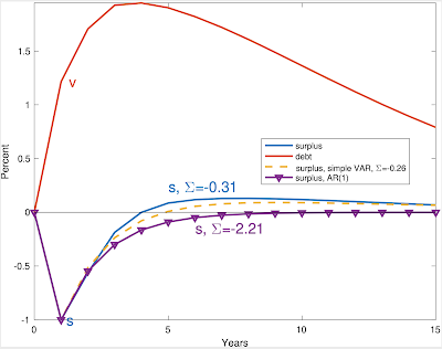
The blue solid line with (s=-0.31) comes from a larger VAR, not shown here. The dashed line comes from the two variable VAR, and the line with triangles comes from the AR(1).

The VAR (dashed line) shows a slight s shape. The moving average coefficients gently turn positive. But when you add it up, those overshootings bring us back to (a(beta)=0.26) despite 5 years of negative responses. (I use (beta=1)). The AR(1) version without debt has (a(beta)=2.21), a factor of 10 larger!

Clearly, whether you include debt in a VAR and find a slightly overshooting moving average, or leave debt out of the VAR and find something like an AR(1) makes a major difference. Which is right? Just as obviously, looking at (R^2)   and t-statistics of the one-step ahead regressions is not going to sort this out.

I now get to the point.

Here are 7 related observations that I think collectively push us to the view that (a(beta)) should be a quite small number. The observations use this very simple model with one period debt and a constant discount rate, but the size and magnitude of the puzzles are so strong that even I don’t think time-varying discount rates can overturn them. If so, well, all the more power to the time-varying discount rate! Again, these observations hold equally for active or passive fiscal policy. This is not about FTPL, at least directly.

1) The correlation of deficits and inflation. Reminder, [ frac{B_{t-1}}{P_{t-1}}Delta E_{t}left( frac{P_{t-1}}{P_{t}}right) =a(beta)varepsilon_{t}. ] If we have an AR(1), (a(beta)=1/(1-rho_{s}beta)approx2), and with (sigma(varepsilon)approx5%) in my little VAR, the AR(1) produces 10% inflation in response to a 1 standard deviation deficit shock. We should see 10% unanticipated inflation in recessions! We see if anything slightly less inflation in recessions, and little correlation of inflation with deficits overall. (a(beta)) near zero solves that puzzle.

2) Inflation volatility. The AR(1) likewise predicts that unexpected inflation has about 10% volatility. Unexpected inflation has about 1% volatility. This observation on its own suggests (a(beta)) no larger than 0.2.

3) Bond return volatility and cyclical correlation. The one-year treasury bill is (so far) completely safe in nominal terms. Thus the volatility and cyclical correlation of unexpected inflation is also the volatility and cyclical correlation of real treasury bill returns. The AR(1) predicts that one-year bonds have a standard deviation of returns around 10%, and they lose in recessions, when the AR(1) predicts a big inflation. In fact one-year treasury bills have no more than 1% standard deviation, and do better in recessions.

4) Mean bond returns. In the AR(1) model, bonds have a stock-like volatility and move procyclically. They should have a stock-like mean return and risk premium. In fact, bonds have low volatility and have if anything a negative cyclical beta so yield if anything less than the risk free rate. A small  (a(beta)) generates low bond mean returns as well.

Jiang, Lustig, Van Nieuwerburgh and Xiaolan recently raised this puzzle, using a VAR estimate of the surplus process that generates a high (a(beta)). Looking at the valuation formula [ frac{B_{t-1}}{P_{t}}=E_{t}sum_{j=0}^{infty}beta^{j}s_{t+j}, ] since surpluses are procyclical, volatile, and serially correlated like dividends, shouldn’t surpluses generate a stock-like mean return? But surpluses are crucially different from dividends because debt is not equity. A low surplus (s_{t}) raises  our estimate of subsequent surpluses (s_{t+j}). If we separate out
 [b_{t}=s_{t}+E_{t}sum_{j=1}^{infty}beta^{j}s_{t+j}=s_{t}+beta E_{t}b_{t+1}  ] a decline in the “cashflow” (s_{t}) raises the “price” term (b_{t+1}), so the overall return is risk free. Bad cashflow news lowers stock pries, so both cashflow and price terms move in the same direction. In sum a small (a(beta)lt 1) resolves the Jiang et. al. puzzle. (Disclosure, I wrote them about this months ago, so this view is not a surprise. They disagree.)

5) Surpluses and debt. Looking at that last equation, with a positively correlated surplus process (a(beta)>1), as in the AR(1), a surplus today leads to  larger value of the debt tomorrow. A deficit today leads to lower value of the debt tomorrow. The data scream the opposite pattern. Higher deficits raise the value of debt, higher surpluses pay down that debt. Cumby_Canzoneri_Diba (AER 2001) pointed this out 20 years ago and how it indicates an s-shaped surplus process.  An (a(beta)lt 1) solves their puzzle as well. (They viewed (a(beta)lt 1) as inconsistent with fiscal theory which is not the case.)

6) Financing deficits. With (a(beta)geq1), the government finances all of each deficit by inflating away outstanding debt, and more. With (a(beta)=0), the government finances deficits by selling debt. This statement just adds up what’s missing from the last one. If a deficit leads to lower value of the subsequent debt, how did the government finance the deficit? It has to be by inflating away outstanding debt. To see this, look again at inflation, which I write [ frac{B_{t-1}}{P_{t-1}}Delta E_{t}left( frac{P_{t-1}}{P_{t}}right) =Delta E_{t}s_{t}+Delta E_{t}sum_{j=1}^{infty}beta^{j}s_{t+j}=Delta E_{t}s_{t}+Delta E_{t}beta b_{t+1}=1+left[ a(beta)-1right] varepsilon_{t}. ] If (Delta E_{t}s_{t}=varepsilon_{t}) is negative — a deficit — where does that come from? With (a(beta)>1), the second term is also negative. So the deficit, and more, comes from a big inflation on the left hand side, inflating away outstanding debt. If (a(beta)=0), there is no inflation, and the second term on the right side is positive — the deficit is financed by selling additional debt. The data scream this pattern as well.

7) And, perhaps most of all, when the government sells debt, it raises revenue by so doing. How is that possible? Only if investors think that higher surpluses will eventually pay off that debt. Investors think the surplus process is s-shaped.

All of these phenomena are tied together.  You can’t fix one without the others. If you want to fix the mean government bond return by, say, alluding to a liquidity premium for government bonds, you still have a model that predicts tremendously volatile and procyclical bond returns, volatile and countercyclical inflation, deficits financed by inflating away debt, and deficits that lead to lower values of subsequent debt.

So, I think the VAR gives the right sort of estimate. You can quibble with any estimate, but the overall view of the world required for any estimate that produces a large (a(beta)) seems so thoroughly counterfactual it’s beyond rescue. The US has persuaded investors, so far, that when it issues debt it will mostly repay that debt and not inflate it all away.

Yes, a moving average that overshoots is a little unusual. But that’s what we should expect from debt. Borrow today, pay back tomorrow. Finding the opposite, something like the AR(1), would be truly amazing. And in retrospect, amazing that so many papers (including my own) write this down. Well, clarity only comes in hindsight after a lot of hard work and puzzles.

In more general settings (a(beta)) above zero gives a little bit of inflation from fiscal shocks, but there are also time-varying discount rates and long term debt in the present value formula. I leave all that to the book and papers.

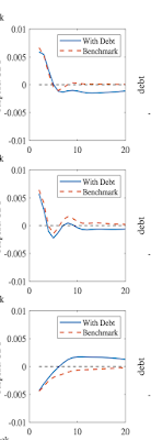
(Jiang et al say they tried it with debt in the VAR and claim it doesn’t make much difference.  But their response functions with debt in the VAR, at left,  show even more overshooting than in my example, so I don’t see how they avoid all the predictions of a small (a(beta)), including a low bond premium.)

A lot of literature on fiscal theory and fiscal sustainability, including my own past papers, used AR(1) or similar surplus processes that don’t allow (a(beta)) near zero. I think a lot of the puzzles that literature encountered comes out of this auxiliary specification. Nothing in fiscal theory prohibits a surplus process with (a(beta)=0) and certainly not (0 lt a(beta)lt 1).

Update

Jiang et al. also claim that it is impossible for any government with a unit root in GDP to issue risk free debt. The hidden assumption is easy to root out. Consider the permanent income model, [ c_t = rk_t + r beta sum beta^j y_{t+j}] Consumption is cointegrated with income and the value of debt. Similarly, we would normally write the surplus process [ s_t = alpha b_t + gamma y_t. ] responding to both debt and GDP. If surplus is only cointegrated with GDP, one imposes ( alpha = 0), which amounts to assuming that governments do not repay debts. The surplus should be cointegrated with GDP and with the value of debt.  Governments with unit roots in GDP can indeed promise to repay their debts.



Source link

قالب وردپرس